Experiment E1610 One Dimensional Constant Acceleration

Figure 1. A ball is dropped and accelerates straight down. Discussion The Model Marking the Video Graphical Analysis

Discussion

Figure 1 shows a picture of a falling ball. In the picture, the horizontal red lines represent the ball's vertical positions at equal time intervals. Notice that the horizontal lines are not evenly spaced as they were in the constant velocity video experiments. This indicates that the velocity is not constant. Therefore, Dv is not zero. And since:

a = Dv/Dt

then there is an acceleration.

Remembering the definition for net force:

F_net = ma

we see that a non-zero acceleration means a non-zero net force.

Therefore, if there is an acceleration, then there must be at least one force causing it. The problem is to identify the forces acting on the object and then experimentally determine if these forces account for the observed acceleration.

Weight:

The first force we will examine is weight. An object's weight (W) depends on its mass (m) and the local gravitational field strength (g). The equation for weight is:

W = mg

Here:

• W is the object's weight in newtons (N).
• m is the object's mass in kilograms (kg).
• g is the local gravitational field strength and has units of N/kg. Close to the earth's surface, g = 9.8 N/kg or 9.8 m/s² as listed in many physics texts. You should verify that N/kg has the same units as m/s².

The characteristics of weight are:

• mg is its magnitude (absolute value).
• its direction is down, toward the earth's center.

Return to Top

The Model

Free Body Diagram:

Physicists use a tool called a free body diagram to illustrate the problem. To draw a free body diagram, follow these steps.

1. Draw the general shape of the object and label it m. This need not be fancy, and in most situations a circle or rectangle is adequate.
2. Pick a positive direction. The positive direction is arbitrary, but once you have chosen it then stay consistent with it.
3. Mentally travel around the object and identify all forces on the object. Draw these forces on the object with arrows indicating the direction of the force and a variable indicating the type of force.

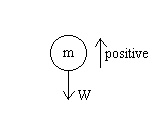
Figure 2 shows a free body diagram for this experiment. Here, the circle with m inside represents the falling ball. The positive direction is show with an upward arrow and the object's weight is represented by a downward arrow with the variable W next to it. The positive direction was chosen up to stay consistent with the computer's definition of up for the positive y direction.

After drawing your diagram then write the equation:

F_net = ma

The left side of this equation is the sum of all the forces that you have placed on your free body diagram, in their correct directions. If a force has the same direction as positive, then it is added on the left side of the net force equation. If a force has the opposite direction as positive, then it is subtracted on the left side of the net force equation. For the free body diagram shown, the net force equation becomes:

-W = ma

Now since W = mg, we can re-write this equation as:

-mg = ma

And dividing both sides by m we have:

-g = a

Our free body diagram analysis has predicted that the object's acceleration will be -g or -9.8 m/s². If this analysis is correct, then this will be the experimental acceleration.

Equations for constant acceleration:

The one dimensional equations for constant acceleration in the y direction are:

1. y = y_o+ v_ot + 0.5at²
2. D = v_ot + 0.5at²
3. v = v_o + at
4. p = mv = m(v_o + at) = mv_o + mat = p_o + F_nett
5. F_net = ma

Notice that if you know y_o, v_o, a, and m, then you can write all these equations.

Remember:

a = Dv/Dt is the definition for acceleration in terms of velocity and time. In words, the acceleration is the slope of a velocity-versus-time graph. The units of acceleration are the units of velocity divided by the units of time. This is m/s/s or m/s².

The velocity equation above is a linear equation with a slope of acceleration (a) and an intercept of v_o. This is straight forward, but where does the displacement equation come from? We'll see if we can derive it using Figure 3, a general linear velocity-versus-time graph.

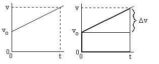
Figure 3 shows a linear velocity-versus-time plot on the left, and the same plot on the right divided into two areas. The triangle has an area of 0.5(height)(base). Here, the height is Dv and the base is t. The rectangle has an area of (height)(base). Here, the height is v_o and the base is also t. The total area is the area of the triangle plus the area of the rectangle. Examining these areas we have:

Total area = v_o^.t + 0.5Dv^.t

Multiplying the last term by t/t we get:

Total area = v_o^.t + 0.5(Dv/t)^.t^.t

Or:

Total area = v_ot + 0.5at²

This is true since (Dv/t) is the acceleration and t^.t is t². Now all terms have units of meters (you should verify this), so this is the object's displacement. The position equation is then easily obtained if you know the initial position.

Return to Top

Marking the Video

1. Play the video and observe the motion.
2. Mark a point on the object until the video does not step any more.
3. What are your observations? Is the object moving in the positive x, negative x, positive y, or negative y direction(s)?
4. Use the Circles - Vectors menu item to observe first the velocity and acceleration and then the momentum and net force. What are your observations?
5. Based on your observations, make rough sketches (no numbers, just the general shape) of the position, displacement, velocity and momentum versus time graphs. Mark the horizontal and vertical axes with the correct variables. You should verify if your sketches are correct when you view these graphs.
6. Looking at your sketch for velocity versus time, will there be an acceleration? If so, will it be positive or negative?
7. Looking at your sketch for momentum versus time, will there be a net force? If so, will it be positive or negative?
8. Draw a free body diagram for this experiment.

Return to Top

Graphical Analysis

Note: To review constant acceleration graphs, run the Graph Tutor software that came on this CD.

1. Press the GRAPHS Button and the Data Analysis Choices will appear. Pick Option 1, then click the Next button.
2. Direction of Motion? Pick the correct direction of motion based on your observations.
3. From the plots options, select position, velocity and momentum. Click the Next button.
4. The first thing you will see is a cover sheet. Write down the mass.
5. Look at the position-versus-time graph. Is it a straight line? Is the slope constant? Is the velocity constant? Is there an acceleration? Is there a net force acting on the object? Find the initial position.
6. Look at the velocity-versus-time graph. Is it a straight line? Is the slope constant? Is the acceleration constant? Find the slope and intercept, then write equations for position, displacement, velocity, and momentum. Check these equations using their graphs.
7. Look at the momentum-versus-time graph. Is it a straight line? Is the slope constant? Is the net force constant? Find the slope and intercept, then write equations for position, displacement, velocity, and momentum. Check these equations using their graphs.

Return to Top