Experiment E2410 One Dimensional Mass/Spring Systems

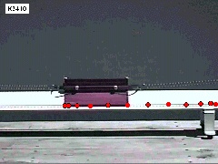
Figure 1. Springs attached to an air glider cause it to oscillate horizontally. Discussion The Model Marking the Video Graphical Analysis

Discussion

When a mass, m, is attached to a spring and displaced from its equilibrium position, then it will oscillate. In other words, the motion of the mass will repeat itself after a specific time. We call this simple harmonic motion with period T. Since the acceleration is not constant, we cannot use the equations for constant acceleration. However, since the motion repeats itself, we might try a sinusoidal function.

Return to Top

The Model

Equations for simple harmonic motion

If the mass oscillates in the x direction, then the equation for x is:

x = x_eq + Acos(q_o + wt)

Here:

• x_eq is the equilibrium position of the mass in meters. This is where the mass is when it is not oscillating.
• A is the maximum distance from the equilibrium position in meters.
• q_o is the phase angle in radians.
• w is the angular frequency in radians/second.
• t is the time in seconds.

The displacement from equilibrium is D_eq = x - x_eq or:

D_eq = Acos(q_o + wt)

The velocity of the mass is:

v = -wAsin(q_o + wt)

And the acceleration of the mass is:

a = -w²Acos(q_o + wt)

Other relationships are:

w = 2p/T

k = mw²

Where T is the period of motion, k is the spring constant, and m is the mass.

If the equation for D_eq above is true then the following equation is also valid.

cos^-1(D_eq/A) = q = q_o + wt

This says that q is a linear function of time with slope w and intercept q_o.

The kinetic and potential energies for a mass/spring system are:

KE = 0.5mv²

PE = 0.5kD_eq²

If the mechanical energy is conserved then:

DKE = -DPE

An Example

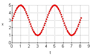
Figure 2 shows a position versus time graph. The maximum value is 5 and the minimum value is 1. Therefore, the equilibrium position is 3 and the amplitude is, A = 2 m. The plot repeats itself every four seconds, therefore the period is, T = 4 s and w = 2p/T = 1.57 rad/s. Placing these values into the position equation at t = 1 s, we have:

x = x_eq + Acos(q_o + wt)

5 = 3 + 2cos(q_o + 1.57(1))

Solving for q_o gives:

q_o = -1.57 radians

We now have all the values we need to write all the equations given at the beginning of this section.

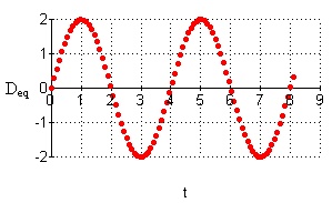
Figure 3 shows a displacement versus time graph. The amplitude is, A = 2 m. The plot repeats itself every four seconds, therefore the period is, T = 4 s and w = 2p/T = 1.57 rad/s. Placing these values into the displacement equation at t = 3 s, we have:

D_eq = Acos(q_o + wt)

-2 = 2cos(q_o + 1.57(3))

Solving for q_o gives:

q_o = -1.57 radians

We now have all the values we need to write all the equations given at the beginning of this section except for the equilibrium position.

Figure 4 was generated using the following equation:

cos^-1(D_eq/A) = q = q_o + wt

Figure 4 is piecewise linear, and we can find q_o and w by finding the intercept and slope of any of the linear segments. Using the first segment, the intercept is about 1.5 and the slope is about -1.5. Therefore we can write:

q_o = 1.5 rad and w = -1.5 rad/s

These values are close to those calculated from Figures 2 and 3, however, they are the negatives of those values. This is a characteristic of the cosine function because:

cos(A) = cos (-A) for all A.

Try using other linear segments from Figure 4 to find q_o and w. Use these values to calculate positions and displacements at various times and check these values using Figures 2 and 3.

Return to Top

Marking the Video

1. Play the video and observe the motion.
2. Mark a position on the mass until the video does not step anymore. If the screen becomes obscured with data points, you can use the menu item Circles then the sub item Show Current to show only the current frame's data point. Using the menu item Circles then the sub item Show All shows all marked data points again.
3. Use the Circles - Vectors menu item to observe first the velocity and acceleration and then the momentum and net force. What are your observations?

Return to Top

Graphical Analysis

Note: To review sinusoidal graphs, run the Graph Tutor software that came on this CD.

1. Press the GRAPHS Button and the Data Analysis Choices will appear. Pick Option 7, then click the Next button.
2. Select position, velocity, acceleration, force, energy, and angle plots. Press the Next button.
3. The cover page appears first. Write down the mass.
4. Analyze the position versus time graph and find the values you need to generate the equations of motion. Write the equations of motion. Check your position equation for at least two times off the position plot.
5. Check your velocity equation for at least two times off the velocity plot.
6. Check your acceleration equation for at least two times off the acceleration plot.
7. Examine the energy versus time plot. Is the total energy conserved? Is the spring force a conservative force? From the data table, create a custom plot of KE versus PE. Find the slope of this plot. What is the physical meaning of this slope?
8. Find the slope and intercept from the angle versus time plot. How do these compare to the values you previously found? Write equations with these values and check your equations against the plots.
9. Analyze the D_eq versus time graph and find the values you need to generate the equations of motion. Write the equations of motion. Check your equations against the plots.
10. From the data table, create a custom plot of D_eq versus v. What is D_eq when v is a maximum? What is D_eq when v is a minimum? What is v when D_eq is a maximum? What is v when D_eq is a minimum?
11. From the data table, create a custom plot of a versus D_eq. Find the slope of this graph. What is the physical significance of this slope?
12. From the data table, create a custom plot of v versus a. What is v when a is a maximum? What is v when a is a minimum? What is a when v is a maximum? What is a when v is a minimum?
13. From the data table, create a custom plot of force versus D_eq. What are the units of the slope of this plot? Look up Hooke's law in any physics text. What is the physical significance of this slope?
14. Does the experiment support the sinusoidal model for a mass/spring system?

Return to Top