The primary obstacle was the lack of independent data. A coaster moving in 3 dimensions requires a minimum of five values to completely describe its motion relative to a stationary observer: the accelerations due to applied forces along the 3 axis and two angles describing its orientation. The data provides information about accelerations but none about orientation.
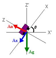
The solution to this problem is to combine the measurements with the constraints of the system. The motion of the coaster can be defined piece wise depending on weather their is a radial acceleration. The mathematics of the 3-D case proved to be far beyond the scope of a introductory physics audience. Fortunately Montazooma's Revenge is essentially restricted to two dimensions. If the movement of the coaster is confined to the x,z plane, all radial acceleration is along the z-axis. Further, any radial acceleration implies a changing normal force due to the changing component of gravity in the z-direction. Similarly, a constant normal force implies no radial acceleration.
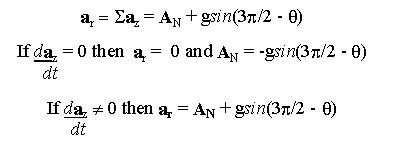
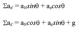
Therefore:
|
|
Finding the angle when there is no radial acceleration is relatively
straight forward. Finding it when the track is curved is not.
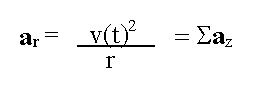
If we substitute an expression for radial acceleration in terms of velocity
and radius into the above equation we get:
Substituting for known quantities and angle as a function of time results
in:
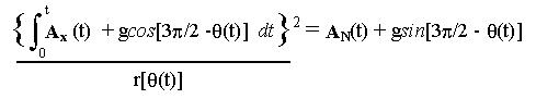
While it may be possible approximate Ax(t) and AN(t) and apply differential calculus to solve for angle as function of time, the techniques needed are far more advanced then plausible for an intro level class. A more feasible method is to step through the data assuming constant accelerations over small intervals of time. Given that we know the initial conditions and we can approximate the angle after a short time, using only linear and rotational kinematics.
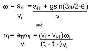
The next angle would be given by:
![]()
Therefore we need the angular acceleration and velocity at a given point.


The next step is to combine the angle with the measured accelerations to find the components of the net acceleration relative to a stationary coordinate system.
|
 |