Experiment E1810 Two Dimensional Constant Acceleration

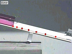
Figure 1. A glider travels on an inclined air track. Discussion The Model Marking the Video Graphical Analysis

Discussion

Figure 1 shows a glider traveling on an inclined air track. From previous experiments, we know that weight will be acting on the glider. But if the weight were the only force, then the glider would accelerate straight down. It does not do this and follows the incline provided by the air track. So, there must be another force acting.

Return to Top

The Model

The Free Body Diagram

Figure 2 shows a drawing and a free body diagram for this experiment. The angle q is the angle of the incline from the horizontal. The right side of the figure shows an x'-y' coordinate system. Here, y' is perpendicular to the incline and x' is parallel to the incline. Notice that the weight has been broken into its components along the x'-y' axes. Also notice the double strike through on the original W vector. This is to remind us not to use it once we have broken it into components. We don't want to add it into our analysis twice.

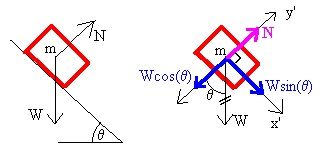
Now, the glider is accelerating down the incline which is the positive x' direction in the figure. Since the normal force is perpendicular to the incline, it cannot cause the acceleration. Remember that the acceleration and the net force must always be in the same direction.

Analyzing the free body diagram in the x' direction we have:

F_netx' = ma_x'

Wsin(q) = ma_x'

mgsin(q) = ma_x'

gsin(q) = a_x'

Our free body diagram analysis has predicted that the object's x' acceleration will be gsin(q). If this analysis is correct, then this will be the experimental acceleration in the x' direction.

It is sometimes useful to look at the extremes. If q is zero, then the incline will be horizontal. And our analysis predicts the acceleration will be zero ( gsin(0^o) = 0). If q is 90^o, then the incline will be vertical. And our analysis predicts the acceleration will be g ( gsin(90^o) = g). Does this make sense?

Analyzing the free body diagram in the y' direction we have:

F_nety' = ma_y'

N - Wcos(q) = ma_y'

But, a_y' is zero so:

N = Wcos(q)

What is N when the incline is horizontal? What is N when the incline is vertical? Do your conclusions make sense?

Now, our analysis suggests that there will be an acceleration in the x' direction. However, the computer has a different coordinate system. How do they relate? Figure 3 shows both the x-y and x'-y' coordinate axes. Notice that the acceleration in the x' direction is at an angle q below the x axis.

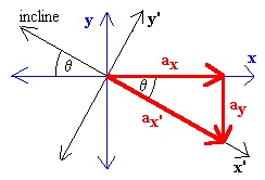
Examining Figure 3 and remembering that a_x' = gsin(q), we see that:

a_x = a_x'cos(q) = gsin(q)cos(q) in the positive x direction.

a_y = a_x'sin(q) = gsin²(q) in the negative y direction.

Therefore, if we can find q then the model predicts the x and y accelerations above.

Two dimensional equations for constant acceleration

Table 1 shows the two dimensional equations for constant acceleration. Notice the similarity to these equations and those for projectile motion. The only difference is the addition of the acceleration terms in the x direction. It would be easy to get the projectile equations from the equations in Table 2 by realizing that a_x is zero.

Table 1. Two dimensional equations for constant acceleration.

Finding the Resultant Vectors

Once you have values for x_o, v_xo, y_o, v_yo, a_x, a_y, and m, then you can write equations for x, y, D_x, D_y, v_x, v_y, p_x, p_y, F_netx, and F_nety as functions of time. You can then substitute a time into any or all of these equations and use your numerical answers to find the resultant vectors at this time. Table 2 summarizes how to find the magnitudes and directions for the vector quantities. Make sure you get the direction in the correct quadrant.

Table 2. Resultant vectors' magnitudes and directions.

Note: In the above table, F_x and F_y have been used instead of F_netx and F_nety for formatting reasons.

Return to Top

Marking the Video

1. Play the video and observe the motion.
2. Move the mouse around on the video and you will notice the x and y positions changing toward the bottom of the screen. Put the mouse on a lower part of the incline and write down the (x,y) location. Put the mouse on a higher part of the incline and write down the (x,y) location. Use these two positions to find the angle of the incline above the horizontal. Then calculate the model's predicted values for a_x', a_x and a_y.
3. Mark a point on the object until the video does not step any more.
4. Examine the vertical and horizontal spacing of the data points. What are your observations?
5. Use the Circles - Vectors menu item to observe first the velocity and acceleration and then the momentum and net force. What are your observations?
6. Based on your observations, make rough sketches (no numbers, just the general shape) of the position, displacement, velocity and momentum versus time graphs. Mark the horizontal and vertical axes with the correct variables. You should verify if your sketches are correct when you view these graphs.

Return to Top

Graphical Analysis

1. Press the GRAPHS Button and the Data Analysis Choices will appear. Pick Option 1, then click the Next button.
2. Direction of Motion? Pick both x and y. Click the Next button.
3. From the plots options, select plots that will allow you to find x_o, v_xo, y_o, v_yo, a_x, and a_y. Click the Next button.
4. The first thing you will see is a cover sheet. Write down the mass.
5. Examine the graphs. Are they the same shape as your sketches?
6. Find the values you need to write equations for the graphs, then check your equations for at least two times.
7. How do the model's predicted accelerations compare to the experimental values? Does this experiment support the model?

Return to Top